[회귀] 다항 회귀 및 과대/과소 적합

1  Polynomial Regression과 오버피팅/언더피팅 이해

• 회귀식이 독립변수의 단항식이 아닌 2차, 3차 방정식과 같은 다항식으로 표현.
• 다항 회귀는 선형 회귀. 선형/비선형 회귀를 나누는 기준은 회귀 계수의 선형/비선형 여부. 독립 변수의 선형/비선형 여부는 무관.

 

1.1  사이킷런에서의 다항 회귀

• 사이킷런에서 다항회귀를 API로 제공하지 않음.
• PolynomialFeatures 클래스로 원본 단항 피처들을 다항 피처들로 변환한 데이터 세트에 LinearRegression 객체를 적용하여 다항회귀 기능 제공.
• PolynomialFeatures : 원본 피처 데이터 세트를 기반으로 degree 차수에 따른 다항식을 적용하여 새로운 피처들을 생성하는 클래스 피처 엔지니어링 기법 중의 하나.
• 사이킷런의 PolynomialFeatures를 사용해 특성의 모든 조합에 대한 교차항을 만드는 것이 좋다. 그 다음 모델 선택 전략을 사용해 최적화된 모델을 만드는 특성 조합과 교차항을 찾는다. 
• 단항 피처를 다항 피처로 변경 한 뒤, LinearRegression 객체로 학습
• 일반적으로 pipeline 클래스를 이용하여 PolynomialFeatures 변환과 LinearRegression 학습/예측을 결합하여 다항 회귀를 구현.

 

1.2  Polynomial Regression 구현

from sklearn.preprocessing import PolynomialFeatures
import numpy as np

# 다항식으로 변환한 단항식 생성, [[0,1],[2,3]]의 2X2 행렬 생성
X = np.arange(4).reshape(2,2)
print('일차 단항식 계수 feature:\n',X )

# degree = 2 인 2차 다항식으로 변환하기 위해 PolynomialFeatures를 이용하여 변환
poly = PolynomialFeatures(degree=2)
poly.fit(X)
poly_ftr = poly.transform(X)
print('변환된 2차 다항식 계수 feature:\n', poly_ftr)

일차 단항식 계수 feature:
[[0 1]
[2 3]]
변환된 2차 다항식 계수 feature:
[[1. 0. 1. 0. 0. 1.]
[1. 2. 3. 4. 6. 9.]]

 

 

from sklearn.linear_model import LinearRegression

def polynomial_func(X):
    y = 1 + 2*X[:,0] + 3*X[:,0]**2 + 4*X[:,1]**3 
    return y

X = np.arange(0,4).reshape(2,2)

print('일차 단항식 계수 feature: \n' ,X)
y = polynomial_func(X)
print('삼차 다항식 결정값: \n', y)

# 3 차 다항식 변환 
poly_ftr = PolynomialFeatures(degree=3).fit_transform(X)
print('3차 다항식 계수 feature: \n',poly_ftr)

# Linear Regression에 3차 다항식 계수 feature와 3차 다항식 결정값으로 학습 후 회귀 계수 확인
model = LinearRegression()
model.fit(poly_ftr,y)
print('Polynomial 회귀 계수\n' , np.round(model.coef_, 2))
print('Polynomial 회귀 Shape :', model.coef_.shape)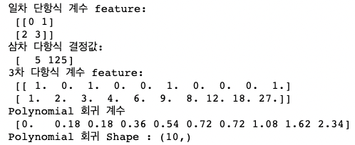

from sklearn.preprocessing import PolynomialFeatures
from sklearn.linear_model import LinearRegression
from sklearn.pipeline import Pipeline
import numpy as np

def polynomial_func(X):
    y = 1 + 2*X[:,0] + 3*X[:,0]**2 + 4*X[:,1]**3 
    return y

# Pipeline 객체로 Streamline 하게 Polynomial Feature변환과 Linear Regression을 연결
model = Pipeline([('poly', PolynomialFeatures(degree=3)),
                  ('linear', LinearRegression())])
X = np.arange(4).reshape(2,2)
y = polynomial_func(X)

model = model.fit(X, y)
print('Polynomial 회귀 계수\n', np.round(model.named_steps['linear'].coef_, 2))

Polynomial 회귀 계수
[0. 0.18 0.18 0.36 0.54 0.72 0.72 1.08 1.62 2.34]

 

1.3  다항 회귀를 이용한 보스턴 주택가격 예측

from sklearn.model_selection import train_test_split
from sklearn.linear_model import LinearRegression
from sklearn.metrics import mean_squared_error , r2_score
from sklearn.preprocessing import PolynomialFeatures
from sklearn.linear_model import LinearRegression
from sklearn.pipeline import Pipeline
import numpy as np
import pandas as pd
from sklearn.datasets import load_boston

# boston 데이타셋 로드
boston = load_boston()

# boston 데이타셋 DataFrame 변환 
bostonDF = pd.DataFrame(boston.data , columns = boston.feature_names)

# boston dataset의 target array는 주택 가격임. 이를 PRICE 컬럼으로 DataFrame에 추가함. 
bostonDF['PRICE'] = boston.target
print('Boston 데이타셋 크기 :',bostonDF.shape)

y_target = bostonDF['PRICE']
X_data = bostonDF.drop(['PRICE'],axis=1,inplace=False)


X_train , X_test , y_train , y_test = train_test_split(X_data , y_target ,test_size=0.3, random_state=156)

## Pipeline을 이용하여 PolynomialFeatures 변환과 LinearRegression 적용을 순차적으로 결합. 
p_model = Pipeline([('poly', PolynomialFeatures(degree=2, include_bias=False)),
                  ('linear', LinearRegression())])

p_model.fit(X_train, y_train)
y_preds = p_model.predict(X_test)
mse = mean_squared_error(y_test, y_preds)
rmse = np.sqrt(mse)


print('MSE : {0:.3f} , RMSE : {1:.3F}'.format(mse , rmse))
print('Variance score : {0:.3f}'.format(r2_score(y_test, y_preds)))

Boston 데이타셋 크기 : (506, 14)
MSE : 15.556 ,
RMSE : 3.944 Variance score : 0.782

 

2  Underfitting (과소 적합) vs. Overfitting (과대 적합)

import numpy as np
import matplotlib.pyplot as plt
from sklearn.pipeline import Pipeline
from sklearn.preprocessing import PolynomialFeatures
from sklearn.linear_model import LinearRegression
from sklearn.model_selection import cross_val_score
%matplotlib inline

# random 값으로 구성된 X값에 대해 Cosine 변환값을 반환. 
def true_fun(X):
    return np.cos(1.5 * np.pi * X)

# X는 0 부터 1까지 30개의 random 값을 순서대로 sampling 한 데이타 입니다.  
np.random.seed(0)
n_samples = 30
X = np.sort(np.random.rand(n_samples))

# y 값은 cosine 기반의 true_fun() 에서 약간의 Noise 변동값을 더한 값입니다. 
y = true_fun(X) + np.random.randn(n_samples) * 0.1

plt.scatter(X, y)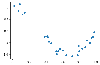

plt.figure(figsize=(14, 5))
degrees = [1, 4, 15]

# 다항 회귀의 차수(degree)를 1, 4, 15로 각각 변화시키면서 비교합니다. 
for i in range(len(degrees)):
    ax = plt.subplot(1, len(degrees), i + 1)
    plt.setp(ax, xticks=(), yticks=())
    
    # 개별 degree별로 Polynomial 변환합니다. 
    polynomial_features = PolynomialFeatures(degree=degrees[i], include_bias=False)
    linear_regression = LinearRegression()
    pipeline = Pipeline([("polynomial_features", polynomial_features),
                         ("linear_regression", linear_regression)])
    pipeline.fit(X.reshape(-1, 1), y)
    
    # 교차 검증으로 다항 회귀를 평가합니다. 
    scores = cross_val_score(pipeline, X.reshape(-1,1), y,scoring="neg_mean_squared_error", cv=10)
    coefficients = pipeline.named_steps['linear_regression'].coef_
    print('\nDegree {0} 회귀 계수는 {1} 입니다.'.format(degrees[i], np.round(coefficients),2))
    print('Degree {0} MSE 는 {1:.2f} 입니다.'.format(degrees[i] , -1*np.mean(scores)))
    
    # 0 부터 1까지 테스트 데이터 세트를 100개로 나눠 예측을 수행합니다. 
    # 테스트 데이터 세트에 회귀 예측을 수행하고 예측 곡선과 실제 곡선을 그려서 비교합니다.  
    X_test = np.linspace(0, 1, 100)
    # 예측값 곡선
    plt.plot(X_test, pipeline.predict(X_test[:, np.newaxis]), label="Model") 
    # 실제 값 곡선
    plt.plot(X_test, true_fun(X_test), '--', label="True function")
    plt.scatter(X, y, edgecolor='b', s=20, label="Samples")
    
    plt.xlabel("x"); plt.ylabel("y"); plt.xlim((0, 1)); plt.ylim((-2, 2)); plt.legend(loc="best")
    plt.title("Degree {}\nMSE = {:.2e}(+/- {:.2e})".format(degrees[i], -scores.mean(), scores.std()))

plt.show()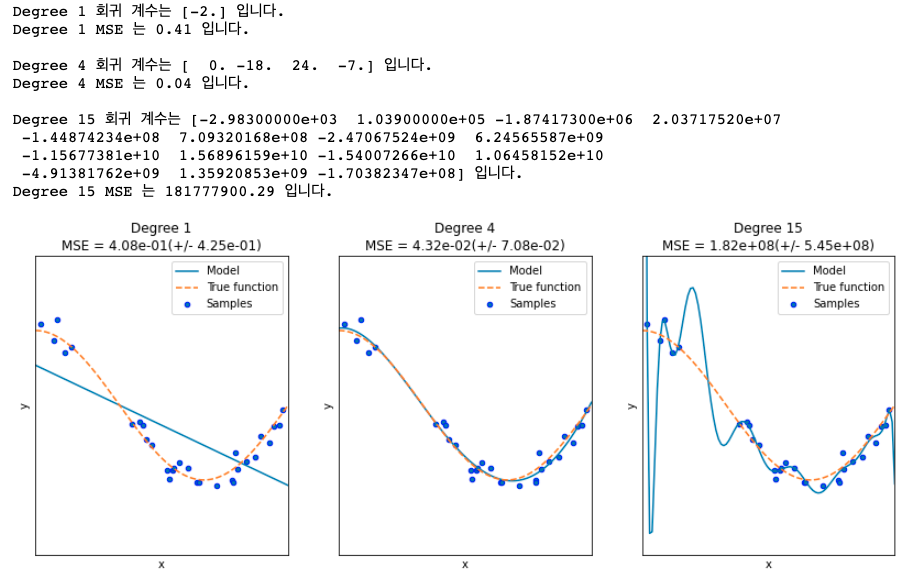

Degree1의 경우 과소 적합. 편향이 굉장히 크다. 편향이 높으면, 분산이 낮음.
Degree15의 경우 과대 적합. 회귀 계수가 지나치게 크게 나와서, 조금만 잘못 계산되도 크게 에러가 난다. 분산이 높으면 편향이 낮아짐.